TransientAnalyzer guide

This notebook shows how to use the TransientAnalyzer

from TransientAnalyzer import TransientAnalyzer
import pandas as pd
import numpy as np
import matplotlib.pyplot as plt

The simulated calcium transients by Tomek et al. 2019 model with the added noise are used as an example

data = np.loadtxt("Transients_SNR10.txt")
T, Ca = data[:,0], data[:,1]

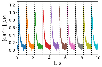
The quality of the signal detection can be checked after initialization of TransientAnalyzer. Individual transients are color-coded and the onset times are displayed. We have also set the first quantile equals to 10% so that the rise and decay time are calculated as 10-90% times of the corresponding phases. There are 100 transients so the total number of transients is detected correctly. The constructor of TransientAnalyzer accepts optionally stimuli times (as one-dimensional numpy array) and quantiles (quantile1 and quantile2) but in this guide we do not provide pre-defined stimuli times and use default percentiles (0.1 and 0.2 respectively).

analyzer = TransientAnalyzer.TransientAnalyzer(T,Ca)
t,ca = analyzer.GetAllExpTransients()
for i in range(len(t)):
    plt.plot(t[i] * 1e-3,ca[i])
for t_null in analyzer.t0s_est:
    plt.axvline(t_null * 1e-3,linestyle="dotted", linewidth = 3, color = 'black')
print(len(analyzer.t0s_est),"transients were detected")
plt.rcParams["font.family"] = "Arial"
plt.xticks(fontsize = 16)
plt.yticks(fontsize = 16)
plt.xlim(0,10)
plt.xlabel('t, s', fontsize = 20)
plt.ylabel('$\mathit{[Ca^{2+}]}, \mu$M', fontsize = 20)
plt.tight_layout()
plt.show()

100 transients were detected

After the detection of all transients, approximate transients and get table with the parameters

analyzer.FitAllTransients()
table = analyzer.GetParametersTable()

Save parameters as excel file

analyzer.ParametersToExcel("params.xlsx",x_label="t, ms",y_label="$\mathit{[Ca^{2+}]}, \mu$M")

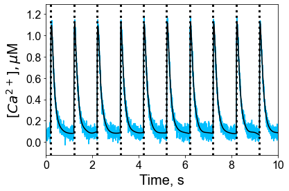
This part shows how to get individual transients, both experimental and approximated ones

t,ca = analyzer.GetAllExpTransients()
for i in range(len(t)):
    T, ca_fit = analyzer.GetApproxTransient(i,1)
    plt.plot(t[i] * 1e-3,ca[i], color="deepskyblue")
    plt.plot(T * 1e-3,ca_fit, color="black")
for t_null in analyzer.t0s:
    plt.axvline(t_null * 1e-3,linestyle="dotted", linewidth = 3, color = 'black')
plt.xticks(fontsize=16)
plt.yticks(fontsize=16)
plt.xlim(0,10)
plt.xlabel('Time, s', fontsize = 20)
plt.ylabel('$\mathit{[Ca^{2+}]}, \mu$M', fontsize = 20)

plt.show()

the recorded data traces as pandas DataFrame. The dataframe contains the parameters written in the documentation of the TransientAnalyzer. This dataframe can be then exported as CSV or Excel file.

traces = analyzer.GetTransientsTable(x_label="t, ms",y_label="$\mathit{[Ca^{2+}]}$, AU")
traces.to_excel("traces.xlsx")